FluidScatteringPlot#
Examples using this class are:
Acoustofluidics 2022: Minimal Example Plotting Scattering Fields
Acoustofluidics 2022: Plotting the Scattering Field


- class osaft.plotting.scattering.fluid_plots.FluidScatteringPlot(sol, r_max, resolution=100, n_quiver_points=21, cmap='winter', div_cmap='coolwarm')[source]#
Bases:
BaseScatteringPlotsClass for plotting scattering field of the fluid
Plots the acoustic field in the fluid around the scatterer using Matplotlib tricontourf or tripcolor plotting methods.
- Parameters:
sol (BaseScattering) – solution to be plotted
r_max (float) – radial limit of plot range
resolution (int | tuple[int, int], optional) – if tuple (radial resolution, tangential resolution)
Default:100n_quiver_points (int, optional) – anchor points along z for quiver
Default:21cmap (str, optional) – color map
Default:'winter'div_cmap (str, optional) – diverging color map
Default:'coolwarm'Public Data Attributes:
Inherited from
BaseScatteringPlotsdataPublic Methods:
plot_velocity_potential([inst, phase, ...])Tricontourf plot for acoustic velocity potential
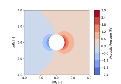
plot_pressure([inst, phase, symmetric, ...])Tricontourf plot for acoustic pressure
plot_velocity([inst, phase, mode, ...])Tricontourf plot for acoustic velocity field of the fluid
animate_pressure([frames, interval, mode, ...])Tricontourf animation for acoustic pressure of the fluid
animate_velocity_potential([frames, ...])Tricontourf animation for acoustic velocity potential of the fluid
animate_velocity([frames, interval, mode, ...])Tricontourf animation for acoustic velocity field of the fluid
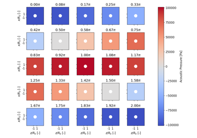
plot_pressure_evolution([inst, mode, ...])Tricontourf for acoustic pressure evolution of the fluid
plot_velocity_potential_evolution([inst, ...])Tricontourf for acoustic velocity potential evolution of the fluid
plot_velocity_evolution([mode, scattered, ...])Tricontourf for acoustic velocity field evolution of the fluid
- animate_pressure(frames=64, interval=100.0, mode=None, scattered=True, incident=True, symmetric=True, tripcolor=False, ax=None, **kwargs)[source]#
Tricontourf animation for acoustic pressure of the fluid
Animates the pressure of the first-order acoustic velocity field of the fluid over one period using Matplotlib’s tricontourf or tripcolor if
tripcolor = True- Parameters:
frames (int, optional) – number of frames for the animation
Default:64interval (float, optional) – interval between frames in ms
Default:100.0mode (None | int, optional) – mode of oscillation
Default:Nonescattered (bool, optional) – if
Truescattering field is plottedDefault:Trueincident (bool, optional) – if
Trueincident field is plottedDefault:Truesymmetric (bool, optional) – if
Truethe symmetry of the solution is usedDefault:Truetripcolor (bool, optional) – switches between tripcolor and tricontourf plot
Default:Falseax (None | plt.Axes, optional) – if
axis passed, plot will be drawn onaxDefault:Nonekwargs – passed through to tricontourf()
- Return type:
FuncAnimation
- animate_velocity(frames=64, interval=100.0, mode=None, scattered=True, incident=True, symmetric=True, quiver_color=None, tripcolor=False, ax=None, **kwargs)[source]#
Tricontourf animation for acoustic velocity field of the fluid
Animates the velocity amplitude of the first-order acoustic velocity field of the fluid over one period using Matplotlib’s tricontourf or tripcolor if
tripcolor = True- Parameters:
frames (int, optional) – number of frames for the animation
Default:64interval (float, optional) – interval between frames in ms
Default:100.0mode (None | int, optional) – mode of oscillation
Default:Nonescattered (bool, optional) – if
Truescattering field is plottedDefault:Trueincident (bool, optional) – if
Trueincident field is plottedDefault:Truesymmetric (bool, optional) – if
Truethe symmetry of the solution is usedDefault:Truequiver_color (None | str, optional) – if not
None, quiver plotDefault:Nonetripcolor (bool, optional) – switches between tripcolor and tricontourf plot
Default:Falseax (None | plt.Axes, optional) – if
axis passed, plot will be drawn onaxDefault:Nonekwargs – passed through to tricontourf()
- Return type:
FuncAnimation
- animate_velocity_potential(frames=64, interval=100.0, mode=None, scattered=True, incident=True, symmetric=True, tripcolor=False, ax=None, **kwargs)[source]#
Tricontourf animation for acoustic velocity potential of the fluid
Animates the velocity potential of the first-order acoustic velocity field of the fluid over one period using Matplotlib’s tricontourf or tripcolor if
tripcolor = True- Parameters:
frames (int, optional) – number of frames for the animation
Default:64interval (float, optional) – interval between frames in ms
Default:100.0mode (None | int, optional) – mode of oscillation
Default:Nonescattered (bool, optional) – if
Truescattering field is plottedDefault:Trueincident (bool, optional) – if
Trueincident field is plottedDefault:Truesymmetric (bool, optional) – if
Truethe symmetry of the solution is usedDefault:Truetripcolor (bool, optional) – switches between tripcolor and tricontourf plot
Default:Falseax (None | plt.Axes, optional) – if
axis passed, plot will be drawn onaxDefault:Nonekwargs – passed through to tricontourf()
- Return type:
FuncAnimation
- plot_pressure(inst=True, phase=0, symmetric=True, mode=None, scattered=True, incident=True, tripcolor=False, ax=None, **kwargs)[source]#
Tricontourf plot for acoustic pressure
Plots the velocity amplitude of the first-order acoustic velocity field of the fluid using Matplotlib’s tricontourf or tripcolor if
tripcolor = True- Parameters:
inst (bool, optional) – if
Trueinstantaneous amplitude is plottedDefault:Truephase (float, optional) – phase \([0, 2\pi]\)
Default:0mode (None | int, optional) – mode of oscillation
Default:Nonescattered (bool, optional) – if
Truescattering field is plottedDefault:Trueincident (bool, optional) – if
Trueincident field is plottedDefault:Truesymmetric (bool, optional) – if
Truethe symmetry of the solution is usedDefault:Truetripcolor (bool, optional) – switches between tripcolor and tricontourf plot
Default:Falseax (None | plt.Axes, optional) – if
axis passed, plot will be drawn onaxDefault:Nonekwargs – passed through to tricontourf()
- Return type:
tuple[plt.Figure, plt.Axes]
- plot_pressure_evolution(inst=True, mode=None, scattered=True, incident=True, symmetric=True, tripcolor=False, layout=(3, 3), **kwargs)[source]#
Tricontourf for acoustic pressure evolution of the fluid
Plots the pressure amplitude of the first-order acoustic pressure field of the fluid over one period at different phases using Matplotlib’s tricontourf or tripcolor if
tripcolor = True.The first phase value is always \(0\pi\) and the last one \(2\pi\). The total number of plots and, hence, also the steps between the different phase values is the defined by the product of the
layouttuple.- Parameters:
inst (bool, optional) – if
Trueinstantaneous amplitude is plottedDefault:Truemode (None | int, optional) – mode of oscillation
Default:Nonescattered (bool, optional) – if
Truescattering field is plottedDefault:Trueincident (bool, optional) – if
Trueincident field is plottedDefault:Truesymmetric (bool, optional) – if
Truethe symmetry of the solution is usedDefault:Truetripcolor (bool, optional) – switches between tripcolor and tricontourf plot
Default:Falselayout (tuple[int, int], optional) – number of rows and columns for plotting
Default:(3, 3)kwargs – passed through to the parent subplots command
- Return type:
tuple[plt.Figure, plt.Axes]
- plot_velocity(inst=True, phase=0, mode=None, scattered=True, incident=True, symmetric=True, quiver_color=None, tripcolor=False, ax=None, **kwargs)[source]#
Tricontourf plot for acoustic velocity field of the fluid
Plots the velocity amplitude of the first-order acoustic velocity field of the fluid using Matplotlib’s tricontourf or tripcolor if
tripcolor = True- Parameters:
inst (bool, optional) – if
Trueinstantaneous amplitude is plottedDefault:Truephase (float, optional) – phase
[0, 2 * pi]Default:0mode (None | int, optional) – mode of oscillation
Default:Nonescattered (bool, optional) – if
Truescattering field is plottedDefault:Trueincident (bool, optional) – if
Trueincident field is plottedDefault:Truesymmetric (bool, optional) – if
Truethe symmetry of the solution is usedDefault:Truetripcolor (bool, optional) – switches between tripcolor and tricontourf plot
Default:Falseax (None | plt.Axes, optional) – if
axis passed, plot will be drawn onaxDefault:Nonekwargs – passed through to tricontourf()
quiver_color (None | str, optional) –
Default:None- Return type:
tuple[plt.Figure, plt.Axes]
- plot_velocity_evolution(mode=None, scattered=True, incident=True, symmetric=True, quiver_color=None, tripcolor=False, layout=(3, 3), **kwargs)[source]#
Tricontourf for acoustic velocity field evolution of the fluid
Plots the velocity amplitude of the first-order acoustic velocity field of the fluid over one period at different phases using Matplotlib’s tricontourf or tripcolor if
tripcolor = True.The first phase value is always \(0\pi\) and the last one \(2\pi\). The total number of plots and, hence, also the steps between the different phase values is the defined by the product of the
layouttuple.- Parameters:
mode (None | int, optional) – mode of oscillation
Default:Nonescattered (bool, optional) – if
Truescattering field is plottedDefault:Trueincident (bool, optional) – if
Trueincident field is plottedDefault:Truesymmetric (bool, optional) – if
Truethe symmetry of the solution is usedDefault:Truequiver_color (None | str, optional) – color of the quiver arrows, if None: no arrows
Default:Nonetripcolor (bool, optional) – switches between tripcolor and tricontourf plot
Default:Falselayout (tuple[int, int], optional) – number of rows and columns for plotting
Default:(3, 3)kwargs – passed through to the parent subplots command
- Return type:
tuple[plt.Figure, plt.Axes]
- plot_velocity_potential(inst=True, phase=0, symmetric=True, mode=None, scattered=True, incident=True, tripcolor=False, ax=None, **kwargs)[source]#
Tricontourf plot for acoustic velocity potential
Plots the velocity amplitude of the first-order acoustic velocity field of the fluid using Matplotlib’s tricontourf or tripcolor if
tripcolor = True- Parameters:
inst (bool, optional) – if
Trueinstantaneous amplitude is plottedDefault:Truephase (float, optional) – phase \([0, 2\pi]\)
Default:0mode (None | int, optional) – mode of oscillation
Default:Nonescattered (bool, optional) – if
Truescattering field is plottedDefault:Trueincident (bool, optional) – if
Trueincident field is plottedDefault:Truesymmetric (bool, optional) – if
Truethe symmetry of the solution is usedDefault:Truetripcolor (bool, optional) – switches between tripcolor and tricontourf plot
Default:Falseax (None | plt.Axes, optional) – if
axis passed, plot will be drawn onaxDefault:Nonekwargs – passed through to tricontourf()
- Return type:
tuple[plt.Figure, plt.Axes]
- plot_velocity_potential_evolution(inst=True, mode=None, scattered=True, incident=True, symmetric=True, tripcolor=False, layout=(3, 3), **kwargs)[source]#
Tricontourf for acoustic velocity potential evolution of the fluid
Plots the velocity potential amplitude of the first-order acoustic velocity potential field of the fluid over one period at different phases using Matplotlib’s tricontourf or tripcolor if
tripcolor = True.The first phase value is always \(0\pi\) and the last one \(2\pi\). The total number of plots and, hence, also the steps between the different phase values is the defined by the product of the
layouttuple.- Parameters:
inst (bool, optional) – if
Trueinstantaneous amplitude is plottedDefault:Truemode (None | int, optional) – mode of oscillation
Default:Nonescattered (bool, optional) – if
Truescattering field is plottedDefault:Trueincident (bool, optional) – if
Trueincident field is plottedDefault:Truesymmetric (bool, optional) – if
Truethe symmetry of the solution is usedDefault:Truetripcolor (bool, optional) – switches between tripcolor and tricontourf plot
Default:Falselayout (tuple[int, int], optional) – number of rows and columns for plotting
Default:(3, 3)kwargs – passed through to the parent subplots command
- Return type:
tuple[plt.Figure, plt.Axes]
- property cmap: str#
Colormap for plotting
- Getter:
return the colormap choice
- Setter:
sets the colormap choice
- property div_cmap: str#
Diverging Colormap for plotting
- Getter:
return the diverging colormap choice
- Setter:
sets the diverging colormap choice