ParticleScatteringPlot#

Examples using this class are:

Scatterer: Acoustic velocity plots with arrows

class osaft.plotting.scattering.particle_plots.ParticleScatteringPlot(sol, resolution=100, n_quiver_points=21, cmap='winter')[source]#

Bases: BaseScatteringPlots

Class for plotting scattering field of the particle

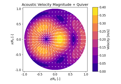
Plots the acoustic field inside the particle using Matplotlib tricontourf or tripcolor plotting methods.

Parameters:

sol (BaseScattering) – solution to be plotted
resolution (int | tuple[int, int], optional) – if tuple (radial resolution, tangential resolution)
Default: 100
n_quiver_points (int, optional) – anchor points along z for quiver
Default: 21
cmap (str, optional) – color map
Default: 'winter'

Public Data Attributes:

Inherited from BaseScatteringPlots

data

Public Methods:

`plot_velocity`([inst, phase, mode, ...])	Tricontourf plot for acoustic velocity field of the particle
`animate_velocity`([frames, interval, mode, ...])	Tricontourf animation for acoustic velocity field of the particle
`plot_velocity_evolution`([inst, mode, ...])	Tricontourf plot for acoustic velocity field evolution of the particle

animate_velocity(frames=64, interval=100.0, mode=None, displacement=True, symmetric=True, quiver_color=None, tripcolor=False, ax=None, **kwargs)[source]#

Tricontourf animation for acoustic velocity field of the particle

Animates the velocity amplitude of the first-order acoustic velocity field of the particle over one period using Matplotlib’s tricontourf or tripcolor if tripcolor = True.

Parameters:

frames (int, optional) – number of frames for the animation
Default: 64
interval (float, optional) – interval between frames in ms
Default: 100.0
mode (None | int, optional) – mode of oscillation
Default: None
displacement (bool, optional) – if True displacement, else velocity plot
Default: True
symmetric (bool, optional) – if True the symmetry of the solution is used
Default: True
quiver_color (None | str, optional) – color of the quiver arrows, if None: no arrows
Default: None
tripcolor (bool, optional) – switches between tripcolor and tricontourf plot
Default: False
ax (None | plt.Axes, optional) – Axes object
Default: None
kwargs – passed through to tricontourf()

Return type:

FuncAnimation

plot_velocity(inst=True, phase=0, mode=None, displacement=False, symmetric=True, quiver_color=None, tripcolor=False, ax=None, **kwargs)[source]#

Tricontourf plot for acoustic velocity field of the particle

Plots the velocity amplitude of the first-order acoustic velocity field of the particle using Matplotlib’s tricontourf or tripcolor if tripcolor = True.

Parameters:

inst (bool, optional) – if True instantaneous amplitude is plotted
Default: True
phase (float, optional) – phase \([0, 2\pi]\)
Default: 0
mode (None | int, optional) – mode of oscillation
Default: None
displacement (bool, optional) – if True displacement, else velocity plot
Default: False
symmetric (bool, optional) – if True the symmetry of the solution is used
Default: True
quiver_color (None | str, optional) – color of the quiver arrows, if None: no arrows
Default: None
tripcolor (bool, optional) – switches between tripcolor and tricontourf plot
Default: False
ax (None | plt.Axes, optional) – Axes object
Default: None
kwargs – passed through to tricontourf()

Return type:

tuple[plt.Figure, plt.Axes]

plot_velocity_evolution(inst=True, mode=None, displacement=False, symmetric=True, quiver_color=None, tripcolor=False, layout=(3, 3), **kwargs)[source]#

Tricontourf plot for acoustic velocity field evolution of the particle

Plots the velocity amplitude of the first-order acoustic velocity field of the fluid over one period at different phases using Matplotlib’s tricontourf or tripcolor if tripcolor = True.

The first phase value is always \(0\pi\) and the last one \(2\pi\). The total number of plots and, hence, also the steps between the different phase values is the defined by the product of the layout tuple.

Parameters:

inst (bool, optional) – if True instantaneous amplitude is plotted
Default: True
mode (None | int, optional) – mode of oscillation
Default: None
displacement (bool, optional) – if True displacement, else velocity plot
Default: False
symmetric (bool, optional) – if True the symmetry of the solution is used
Default: True
quiver_color (str, optional) – color of the quiver arrows, if None: no arrows
Default: None
tripcolor (bool, optional) – switches between tripcolor and tricontourf plot
Default: False
layout (tuple[int, int], optional) – number of rows and columns for plotting
Default: (3, 3)
kwargs – passed through to the parent subplots command

Return type:

tuple[plt.Figure, plt.Axes]