Acoustofluidics 2022: ARF Comparison

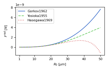
In this example, we reproduce the ARF comparison plot from the abstract book for the conference Acoustofluidics 2022. We compute the ARF on a polystyrene particle in a standing wave in water.

We start off by importing the library and defining all the necessary parameters.

import numpy as np
from matplotlib import pyplot as plt

import osaft

# Frequency
f = 5e6  # [Hz]
# Radius
R_0 = 1e-6  # [m]
# Density and speed of sound of polystyrene
rho_s = 1020  # [kg/m^3]
c_s = 2_350  # [m/s]
# Density and speed of sound of the fluid
rho_f = 997  # [kg/m^3]
c_f = 1_498  # [m/s]
# Pressure amplitude
p_0 = 1e5  # [Pa]
# Particle position
d = osaft.pi / 4
# Wave Type
wave_type = osaft.WaveType.STANDING

For this example we compare three inviscid theories. The models by Yosioka & Kawasima and the model by Gor’kov assume a fluid-like, compressible particle. The latter model is restricted to the long-wavelength regime. The model from Hasegawa & Yosioka assume a solid-elastic particle.

# Model from Yosioka & Kawasima
yosioka = osaft.yosioka1955.ARF(
    f=f, R_0=R_0,
    rho_s=rho_s, c_s=c_s,
    rho_f=rho_f, c_f=c_f,
    p_0=p_0, wave_type=wave_type,
    position=d,
)

# Model from Gor'kov
gorkov = osaft.gorkov1962.ARF(
    f=f, R_0=R_0,
    rho_s=rho_s, c_s=c_s,
    rho_f=rho_f, c_f=c_f,
    p_0=p_0, wave_type=wave_type,
    position=d,
)

Elastic properties of polystyrene for the model of Hasegawa & Yosioka are matched to the compressibility of the other two models.

nu_s = 0.4  # [-]
E_s = 3 * (1 - 2 * nu_s) / yosioka.scatterer.kappa_f  # [Pa]

hasegawa = osaft.hasegawa1969.ARF(
    f=f, R_0=R_0,
    rho_s=rho_s, E_s=E_s, nu_s=nu_s,
    rho_f=rho_f, c_f=c_f,
    p_0=p_0, wave_type=wave_type,
    position=d,
)

Next, we plot the ARF according to the theories while changing the radius of the particle. For a more detailed explanation how this is done checkout this example. For a small particle radius, the models are in good agreement. When the particle becomes larger the model by Gor’kov is no longer valid. Also the other two models are no longer in good agreement. The material model of the particle seems to strongly influence the ARF as higher order modes start to contribute more significantly. To see an animation of these modes checkout this example.

# Changing the font size in Matplotlib
plt.rcParams.update({'font.size': 8})

# Getting a Figure, Axes instance with the right size
fig, ax = plt.subplots(figsize=(3.7, 2.4))

# Plot using the Axes object created above
arf_plot = osaft.ARFPlot('R_0', np.linspace(1e-6, 50e-6, 100))
arf_plot.add_solutions(gorkov, yosioka, hasegawa)
arf_plot.plot_solutions(ax=ax)

# Changing labels
ax.set_xlabel('$R_0$ [$\\mu m$]')
ax.set_ylabel('$F^{rad}$ [$N$]')
ax.set_xticks(
    [1e-6, 1e-5, 2e-5, 3e-5, 4e-5, 5e-5],
    labels=[1, 10, 20, 30, 40, 50],
)

# Adjust layout and display plot
fig.tight_layout()
plt.show()

/home/docs/checkouts/readthedocs.org/user_builds/osaft/checkouts/patch-doinikov2021_streaming/osaft/plotting/datacontainers/arf_datacontainer.py:52: AssumptionWarning: Theory might not be valid anymore!
  self._arf = self._compute_arf_single_process(attr_name, values)

Estimated memory usage: 10 MB