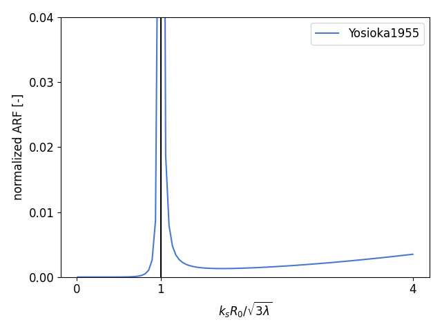
Yosioka and Kawasima (1955) Figure 2

With this example we want to recreate Figure 2 from the publication of Yosioka and Kawasima (1955).

First, we need to get an instance of our solution class. In this case osaft.yosioka1955.ARF(). The steps are the same as in the earlier examples.

import matplotlib.pyplot as plt
import numpy as np

import osaft

# --------
# Geometry
# --------
# Radius
R_0 = 1e-6  # [m]

# -----------------
# Properties of Air
# -----------------
# Speed of sound
c_air = 343  # [m/s]
# Density
rho_air = 1.225  # [kg/m^3]

# -------------------
# Properties of Water
# -------------------
# Speed of sound
c_w = 1_498  # [m/s]
# Density
rho_w = 997  # [kg/m^3]

# --------------------------------
# Properties of the Acoustic Field
# --------------------------------
# Frequency
f = 1e5  # [Hz]
# Pressure
p_0 = 101_325  # [Pa]
# Wave type
wave_type = osaft.WaveType.TRAVELLING

# Initializing Model Instance
yosioka = osaft.yosioka1955.ARF(
    f=f,
    R_0=R_0,
    rho_s=rho_air, c_s=c_air,
    rho_f=rho_w, c_f=c_w,
    p_0=p_0,
    wave_type=wave_type,
    bubble_solution=True,
    small_particle=True,
)

For this example we are plotting the acoustic radiation for against

\[44x(R_0) = k_s * R_0 / \sqrt{3 \tilde{\rho}}\]

where \(k_s\) is the wavenumber in the bubble, \(R_0\) is the radius, and \(\tilde{\rho}\) is the ratio of the particle density and the fluid density. \(x(R_0)\) is ranging between 0 and 4. We, therefore, need to compute the values of \(R_0\) takes, such that \(x(R_0)\) is in this range.

x_values = np.linspace(0.01, 4, num=100)
x_values = np.append(x_values, 1)
x_values = np.sort(x_values)

R_values = x_values * np.sqrt(3 * yosioka.rho_s / yosioka.rho_f) / yosioka.k_s

Now that we have the values on the x-axis, we can plot the ARF. We pass normalization_name = 'max'. This will normalize the ARF w.r.t. the max value in the plot.

# Plotting the acoustic radiation force with osaft
arf_plot = osaft.ARFPlot()
arf_plot.add_solutions(yosioka)
arf_plot.set_abscissa(x_values=R_values, attr_name='R_0')
fig, ax = arf_plot.plot_solutions(display_values=x_values, normalization='max')

# Finally, we manipulate the Axes object to make it more similar to the plot
# in the paper.

# adding a black vertical line at x = 1
ax.axvline(1, color='k')

# setting the x-axis ticks
ax.set_xticks([0, 1, 4])

# setting y-axis limits and the ticks
ax.set_ylim(0, 0.04)
ax.set_yticks([0, 0.01, 0.02, 0.03, 0.04])

# adding labels to both axis
ax.set_xlabel(r'${k_s R_0}/{\sqrt{3\lambda}}$')

# displaying the plot
fig.tight_layout()
plt.show()

# sphinx_gallery_thumbnail_number = -1

/home/docs/checkouts/readthedocs.org/user_builds/osaft/checkouts/patch-doinikov2021_streaming/osaft/plotting/datacontainers/arf_datacontainer.py:52: AssumptionWarning: Theory might not be valid anymore!
  self._arf = self._compute_arf_single_process(attr_name, values)

Estimated memory usage: 9 MB