Doinikov 2021 Viscous - Convergence Study

In this example we use the model doinikov2021viscous. For the computation of the ARF the acoustic field is integrated from the surface of the particle to infinity. “Infinity” here means a point far away from the particle where the acoustic field is no longer influenced by its presence. Our quadrature method scipy.integrate.quad offers the option to integrate to infinity for converging functions. However, for the given integral this does not work reliably. We therefore choose the distance far away from the particle ourselves. In this example it is shown how.

In this example we study a glass sphere viscous fluid.

import numpy as np
from matplotlib import pyplot as plt

import osaft

# --------
# Geometry
# --------
# Radius
R_0 = 1e-6  # [m]

# --------------------
# Properties of Glass
# --------------------
# Speed of sound
c_1_glass = 4_521  # [m/s]
c_2_glass = 2_226  # [m/s]
# Density
rho_glass = 2_240  # [kg/m^3]

# -----------------
# Properties of Oil
# -----------------
# Speed of sound
c_oil = 1_400  # [m/s]
# Density
rho_oil = 900  # [kg/m^3]
# Viscosity
eta_oil = 0.04  # [Pa s]
zeta_oil = 0  # [Pa s]

# --------------------------------
# Properties of the Acoustic Field
# --------------------------------
# Frequency
f = 5e5  # [Hz]
# Pressure
p_0 = 1e5  # [Pa]
# Wave type
wave_type = osaft.WaveType.STANDING
# Position of the particle in the field
position = np.pi / 4  # [rad]

Here, we are given the primary and the secondary wave speed of glass only. The model doinikov2021viscous, however, takes the Young’s modulus and the Poisson’s ratio as input parameters. We therefore have to convert the properties. The ElasticSolid class offers such conversion methods.

E_s = osaft.ElasticSolid.E_from_wave_speed(c_1_glass, c_2_glass, rho_glass)
nu_s = osaft.ElasticSolid.nu_from_wave_speed(c_1_glass, c_2_glass)

doinikov_viscous = osaft.doinikov2021viscous.ARF(
    f=f, R_0=R_0,
    rho_s=rho_glass, E_s=80e9, nu_s=0.20,
    rho_f=rho_oil, c_f=c_oil,
    eta_f=eta_oil, zeta_f=zeta_oil,
    p_0=p_0, wave_type=wave_type,
    position=position,
    inf_factor=60, inf_type=None,
)

We could now straightaway compute the ARF with the model. And for most cases this will work just fine. However, if you need to be extra sure that the integral has been solved accurately you might want to make a conversion study for the value of “infinity”. By default, this value is set to \(60\max{(R_0,\delta)}\). That is, it is set to 60 times the boundary layer thickness or the radius, whichever is greater.

print(f'{doinikov_viscous.R_0 = }')
print(f'{doinikov_viscous.delta = }')
print(f'{doinikov_viscous.inf_factor = }')
print(f'{doinikov_viscous.inf = }')

doinikov_viscous.R_0 = 1e-06
doinikov_viscous.delta = 5.319230405352436e-06
doinikov_viscous.inf_factor = 60
doinikov_viscous.inf = 0.00031915382432114614

The value of inf can also be set manually using the two parameters inf_factor and inf_type. inf_factor is the prefactor for inf_type and should be a numerical value. For inf_type there are 4 options:

• None: \(\text{inf_factor}\cdot\max{(R_0,\delta)}\)

• 'delta': the boundary layer thickness \(\delta\)

• 'radius': the radius \(\delta\)

• 1 or '1': inf is simply the inf_factor

Usually leaving it at None is the best option.

doinikov_viscous.inf_type = 1
doinikov_viscous.inf_factor = 1e-4
print(f'{doinikov_viscous.inf_factor = }')
print(f'{doinikov_viscous.inf_type = }')
print(f'{doinikov_viscous.inf = }')
doinikov_viscous.inf_type = 'radius'
doinikov_viscous.inf_factor = 60
print(f'{doinikov_viscous.inf_factor = }')
print(f'{doinikov_viscous.inf_type = }')
print(f'{doinikov_viscous.inf = }')

doinikov_viscous.inf_factor = 0.0001
doinikov_viscous.inf_type = 1
doinikov_viscous.inf = 0.0001
doinikov_viscous.inf_factor = 60
doinikov_viscous.inf_type = 'radius'
doinikov_viscous.inf = 5.9999999999999995e-05

Often it is not apriori clear what value should be chosen. Therefore, a convergence study can be performed. The plotting functionality of OSAFT can be very handy for this since we can plot the ARF against the inf_factor.

In order for multiprocessing to work you need to run your code inside the if __name__ == '__main__': clause as shown below. Check the multiprocessing example.

if __name__ == '__main__':

    doinikov_viscous.inf_type = None
    plot = osaft.ARFPlot('inf_factor', np.arange(10, 200, 30))
    plot.add_solutions(doinikov_viscous, multicore=True)
    fig, ax = plot.plot_solutions(normalization='max', marker='o')

    ax.set_xlabel('inf_factor')
    ax.ticklabel_format(useOffset=False)
    fig.tight_layout()
    plt.show()

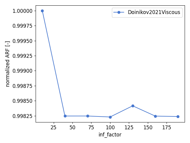
We see that already for a value of inf_factor of 40 the ARF stops changing significantly. In fact, going from inf_factor = 40 to inf_factor = 200 will change the value of the ARF less than 0.001%. This will be sufficiently accurate for most cases. Note that this also means for the given example the default settings would give a very accurate estimate of the ARF.

Estimated memory usage: 9 MB