Note
Go to the end to download the full example code
Pressure Plot
This examples shows you how to plot the pressure field.
As always we start off by importing the necessary Python modules. For our example we are going to need the osaft library, and the third party package Matplotlib.
13 from matplotlib import pyplot as plt
14
15 import osaft
The next step is to define the properties for our example, these include the material properties, the properties of the acoustic field and the radius. We always assume SI-units.
The wave type is set using the osaft.WaveType enum. Currently, there are
two options:
osaft.WaveType.STANDING and osaft.WaveType.TRAVELLING for a plane
standing wave and a plane travelling wave, respectively.
28 # --------
29 # Geometry
30 # --------
31 # Radius
32 R_0 = 5e-6  # [m]
33
34 # -----------------
35 # Properties of copper
36 # -----------------
37 # Density
38 rho_cu = 8960  # [kg/m^3]
39 # Young's modulus
40 E_cu = 130e9  # [Pa]
41 # Possion ratio
42 nu_cu = 0.34  # [-]
43
44 # -------------------
45 # Properties of Water
46 # -------------------
47 # Speed of sound
48 c_w = 1_498  # [m/s]
49 # Density
50 rho_w = 997  # [kg/m^3]
51
52 # --------------------------------
53 # Properties of the Acoustic Field
54 # --------------------------------
55 # Frequency
56 f = 5e5  # [Hz]
57 # Pressure
58 p_0 = 1e5  # [Pa]
59 # Wave type
60 wave_type = osaft.WaveType.STANDING
61 # Position of the particle in the field
62 position = osaft.pi / 4  # [rad]
Once all properties are defined we can initialize the solution instances for the scattering field. In this case we are using the model Hasegawa (1969). However, you can also chose any other model that has the scattering implemented.
70 sol = osaft.hasegawa1969.ScatteringField(
71     f=f,
72     R_0=R_0,
73     rho_s=rho_cu,
74     E_s=E_cu, nu_s=nu_cu,
75     rho_f=rho_w, c_f=c_w,
76     p_0=p_0,
77     wave_type=wave_type,
78     position=position,
79 )
The next step is to initialise the plotter
83 plotter = osaft.FluidScatteringPlot(sol, r_max=5 * sol.R_0)
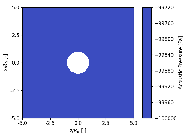
In the first step we want to check if the set input pressure of p_0=1e5
matches with the calculated incident pressure field. Since we are in a
standing wave field and will look at the time zero. We set the position to a
multiple of osaft.pi such that we are the pressure maximum or minimum
92 sol.position = 0
93
94 fig, _ = plotter.plot_pressure(
95     inst=True, tripcolor=False,
96     incident=True, scattered=False,
97 )
98 fig.tight_layout()
99 plt.show()
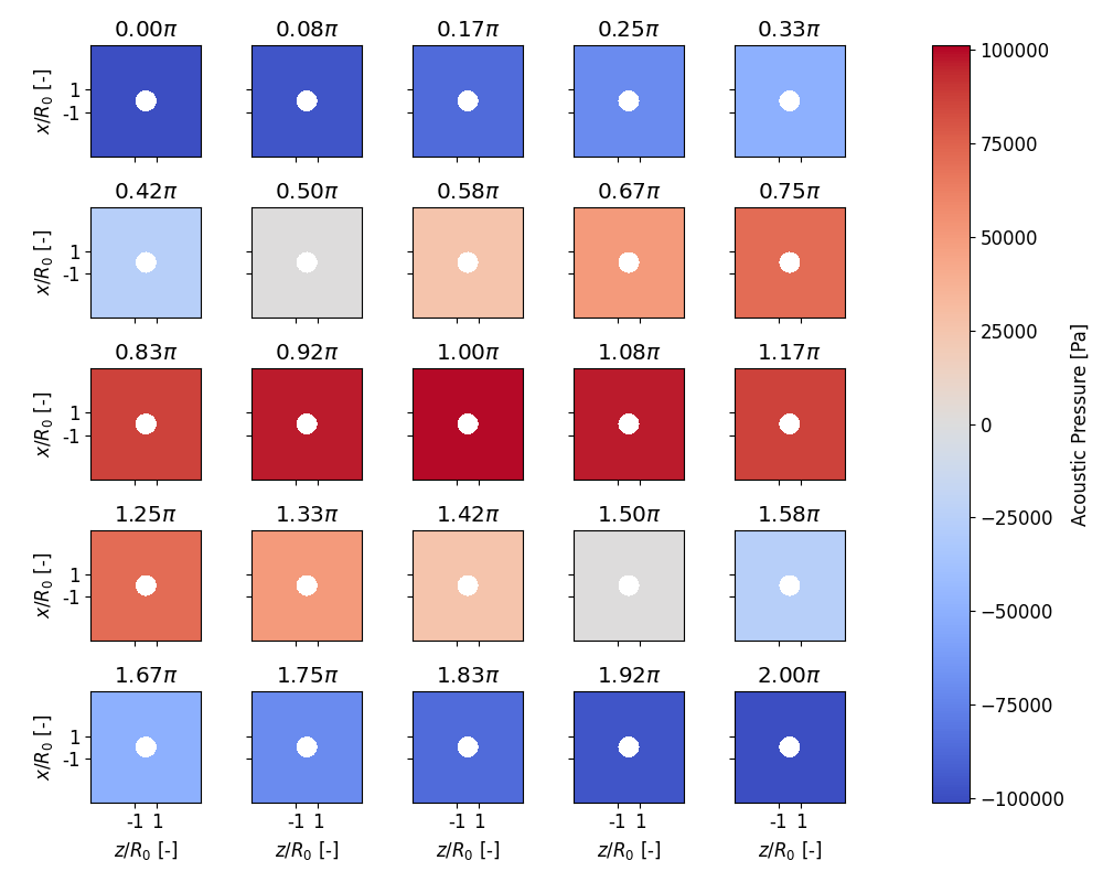
Alternatively, we can also look in an evolution plot how the pressure field
evolves for different phase values. The default layout is 3x3 and can be
adjusted with the option layout=(n_row, n_cols). Additionally we increase
the figure size with figsize=(...) to enlarge the plots.
107 # sphinx_gallery_thumbnail_number = 2
108
109 plotter.plot_pressure_evolution(
110     inst=True, tripcolor=False,
111     layout=(5, 5), figsize=(10, 8),
112     incident=True, scattered=False,
113 )
114 plt.show()
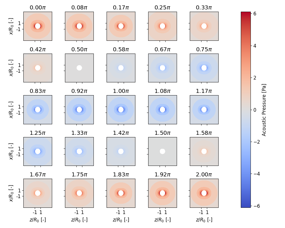
Now lets see what the magnitude of the scattered field is
119 plotter.plot_pressure_evolution(
120     inst=True, tripcolor=False,
121     layout=(5, 5), figsize=(10, 8),
122     incident=False, scattered=True,
123 )
124 plt.show()
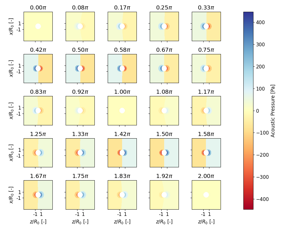
We might be also wondering how it looks for a travelling wave. Additionally,
we can change the colormap. Note here, that we set the attribute
plotter.div_cmap since the data that will be plotted will contain
positive and negative values. Also, it is useful to have a diverging colormap
that is NOT white in the center because the scatterer is depicted white in
our plots.
134 sol.wave_type = osaft.WaveType.TRAVELLING
135 plotter.div_cmap = 'RdYlBu'
136
137 plotter.plot_pressure_evolution(
138     inst=True, tripcolor=False,
139     layout=(5, 5), figsize=(10, 8),
140     incident=False, scattered=True,
141 )
142 plt.show()
Lastly we want to animate the pressure. Keep in mind that now the wave type is travelling
148 anim = plotter.animate_pressure(scattered=True, incident=False)
149 anim.resume()
150 plt.show()
Total running time of the script: ( 1 minutes 51.482 seconds)
Estimated memory usage: 9 MB