FluidScatteringPlot
Examples using this class are:
Acoustofluidics 2022: Minimal Example Plotting Scattering Fields
Acoustofluidics 2022: Plotting the Scattering Field
- class osaft.plotting.scattering.fluid_plots.FluidScatteringPlot(sol, r_max, theta_min=0, theta_max=3.141592653589793, resolution=100, cmap='winter', div_cmap='coolwarm')[source]
Bases:
objectClass for plotting scattering field of the fluid
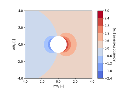
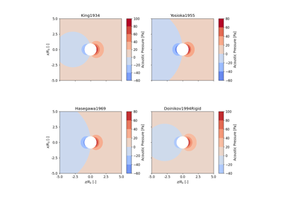
Plots the acoustic field around the particle using Matplotlib tricontourf or tripcolor plotting methods.
- Parameters:
sol (
BaseScattering) – solution to be plottedr_max (
float) – radial limit of plot rangetheta_min (
float, optional) – lower limit for tangential plot rangeDefault:0theta_max (
float, optional) – upper limit for tangential plot rangeDefault:3.141592653589793resolution (
Union[int,tuple[int,int]], optional) – if tuple (radial resolution, tangential resolution)Default:100cmap (
str, optional) – color mapDefault:'winter'div_cmap (
str, optional) – diverging color mapDefault:'coolwarm'Public Methods:
plot_velocity_potential([inst, phase, ...])Tricontourf plot for acoustic velocity potential
plot_pressure([inst, phase, symmetric, ...])Tricontourf plot for acoustic pressure
plot_velocity([inst, phase, mode, ...])Tricontourf plot for acoustic velocity field of the fluid
animate_pressure([frames, interval, mode, ...])Tricontourf animation for acoustic pressure of the fluid
animate_velocity_potential([frames, ...])Tricontourf animation for acoustic velocity potential of the fluid
animate_velocity([frames, interval, mode, ...])Tricontourf animation for acoustic velocity field of the fluid
plot_pressure_evolution([inst, mode, ...])Tricontourf for acoustic pressure evolution of the fluid
plot_velocity_potential_evolution([inst, ...])Tricontourf for acoustic velocity potential evolution of the fluid
plot_velocity_evolution([mode, scattered, ...])Tricontourf for acoustic velocity field evolution of the fluid
- animate_pressure(frames=64, interval=100.0, mode=None, scattered=True, incident=True, symmetric=True, tripcolor=False, ax=None, **kwargs)[source]
Tricontourf animation for acoustic pressure of the fluid
Animates the pressure of the first-order acoustic velocity field of the fluid over one period using Matplotlib’s tricontourf or tripcolor if
tripcolor = True- Parameters:
frames (
int, optional) – number of frames for the animationDefault:64interval (
float, optional) – interval between frames in msDefault:100.0mode (
Optional[int], optional) – mode of oscillationDefault:Nonescattered (
bool, optional) – ifTruescattering field is plottedDefault:Trueincident (
bool, optional) – ifTrueincident field is plottedDefault:Truesymmetric (
bool, optional) – ifTruethe symmetry of the solution is usedDefault:Truetripcolor (
bool, optional) – switches between tripcolor and tricontourf plotDefault:Falseax (
Optional[Axes], optional) – Axes objectDefault:Nonekwargs – passed through to tricontourf()
- Return type:
- animate_velocity(frames=64, interval=100.0, mode=None, scattered=True, incident=True, symmetric=True, tripcolor=False, ax=None, **kwargs)[source]
Tricontourf animation for acoustic velocity field of the fluid
Animates the velocity amplitude of the first-order acoustic velocity field of the fluid over one period using Matplotlib’s tricontourf or tripcolor if
tripcolor = True- Parameters:
frames (
int, optional) – number of frames for the animationDefault:64interval (
float, optional) – interval between frames in msDefault:100.0mode (
Optional[int], optional) – mode of oscillationDefault:Nonescattered (
bool, optional) – ifTruescattering field is plottedDefault:Trueincident (
bool, optional) – ifTrueincident field is plottedDefault:Truesymmetric (
bool, optional) – ifTruethe symmetry of the solution is usedDefault:Truetripcolor (
bool, optional) – switches between tripcolor and tricontourf plotDefault:Falseax (
Optional[Axes], optional) – Axes objectDefault:Nonekwargs – passed through to tricontourf()
- Return type:
- animate_velocity_potential(frames=64, interval=100.0, mode=None, scattered=True, incident=True, symmetric=True, tripcolor=False, ax=None, **kwargs)[source]
Tricontourf animation for acoustic velocity potential of the fluid
Animates the velocity potential of the first-order acoustic velocity field of the fluid over one period using Matplotlib’s tricontourf or tripcolor if (w.*)
- Parameters:
frames (
int, optional) – number of frames for the animationDefault:64interval (
float, optional) – interval between frames in msDefault:100.0mode (
Optional[int], optional) – mode of oscillationDefault:Nonescattered (
bool, optional) – ifTruescattering field is plottedDefault:Trueincident (
bool, optional) – ifTrueincident field is plottedDefault:Truesymmetric (
bool, optional) – ifTruethe symmetry of the solution is usedDefault:Truetripcolor (
bool, optional) – switches between tripcolor and tricontourf plotDefault:Falseax (
Optional[Axes], optional) – Axes objectDefault:Nonekwargs – passed through to tricontourf()
- Return type:
- plot_pressure(inst=True, phase=0, symmetric=True, mode=None, scattered=True, incident=True, tripcolor=False, ax=None, **kwargs)[source]
Tricontourf plot for acoustic pressure
Plots the velocity amplitude of the first-order acoustic velocity field of the fluid using Matplotlib’s tricontourf or tripcolor if
tripcolor = True- Parameters:
inst (
bool, optional) – ifTrueinstantaneous amplitude is plottedDefault:Truephase (
float, optional) – phase [0, 2 * pi]Default:0mode (
Optional[int], optional) – mode of oscillationDefault:Nonescattered (
bool, optional) – ifTruescattering field is plottedDefault:Trueincident (
bool, optional) – ifTrueincident field is plottedDefault:Truesymmetric (
bool, optional) – ifTruethe symmetry of the solution is usedDefault:Truetripcolor (
bool, optional) – switches between tripcolor and tricontourf plotDefault:Falseax (
Optional[Axes], optional) – Axes objectDefault:Nonekwargs – passed through to tricontourf()
- Return type:
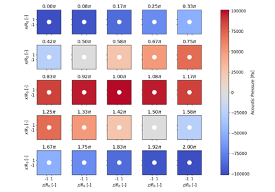
- plot_pressure_evolution(inst=True, mode=None, scattered=True, incident=True, symmetric=True, tripcolor=False, layout=(3, 3), **kwargs)[source]
Tricontourf for acoustic pressure evolution of the fluid
Plots the pressure amplitude of the first-order acoustic pressure field of the fluid over one period at different phases using Matplotlib’s tricontourf or tripcolor if (w.*).
The first phase value is always \(0\pi\) and the last one \(2\pi\). The total number of plots and, hence, also the steps between the different phase values is the defined by the product of the
layouttuple.- Parameters:
inst (
bool, optional) – ifTrueinstantaneous amplitude is plottedDefault:Truemode (
Optional[int], optional) – mode of oscillationDefault:Nonescattered (
bool, optional) – ifTruescattering field is plottedDefault:Trueincident (
bool, optional) – ifTrueincident field is plottedDefault:Truesymmetric (
bool, optional) – ifTruethe symmetry of the solution is usedDefault:Truetripcolor (
bool, optional) – switches between tripcolor and tricontourf plotDefault:Falselayout (
tuple[int,int], optional) – number of rows and columns for plottingDefault:(3, 3)kwargs – passed through to the parent subplots command
- Return type:
- plot_velocity(inst=True, phase=0, mode=None, scattered=True, incident=True, symmetric=True, tripcolor=False, ax=None, **kwargs)[source]
Tricontourf plot for acoustic velocity field of the fluid
Plots the velocity amplitude of the first-order acoustic velocity field of the fluid using Matplotlib’s tricontourf or tripcolor if
tripcolor = True- Parameters:
inst (
bool, optional) – ifTrueinstantaneous amplitude is plottedDefault:Truephase (
float, optional) – phase [0, 2 * pi]Default:0mode (
Optional[int], optional) – mode of oscillationDefault:Nonescattered (
bool, optional) – ifTruescattering field is plottedDefault:Trueincident (
bool, optional) – ifTrueincident field is plottedDefault:Truesymmetric (
bool, optional) – ifTruethe symmetry of the solution is usedDefault:Truetripcolor (
bool, optional) – switches between tripcolor and tricontourf plotDefault:Falseax (
Optional[Axes], optional) – Axes objectDefault:Nonekwargs – passed through to tricontourf()
- Return type:
- plot_velocity_evolution(mode=None, scattered=True, incident=True, symmetric=True, tripcolor=False, layout=(3, 3), **kwargs)[source]
Tricontourf for acoustic velocity field evolution of the fluid
Plots the velocity amplitude of the first-order acoustic velocity field of the fluid over one period at different phases using Matplotlib’s tricontourf or tripcolor if
tripcolor = True.The first phase value is always \(0\pi\) and the last one \(2\pi\). The total number of plots and, hence, also the steps between the different phase values is the defined by the product of the
layouttuple.- Parameters:
mode (
Optional[int], optional) – mode of oscillationDefault:Nonescattered (
bool, optional) – ifTruescattering field is plottedDefault:Trueincident (
bool, optional) – ifTrueincident field is plottedDefault:Truesymmetric (
bool, optional) – ifTruethe symmetry of the solution is usedDefault:Truetripcolor (
bool, optional) – switches between tripcolor and tricontourf plotDefault:Falselayout (
tuple[int,int], optional) – number of rows and columns for plottingDefault:(3, 3)kwargs – passed through to the parent subplots command
- Return type:
- plot_velocity_potential(inst=True, phase=0, symmetric=True, mode=None, scattered=True, incident=True, tripcolor=False, ax=None, **kwargs)[source]
Tricontourf plot for acoustic velocity potential
Plots the velocity amplitude of the first-order acoustic velocity field of the fluid using Matplotlib’s tricontourf or tripcolor if
tripcolor = True- Parameters:
inst (
bool, optional) – ifTrueinstantaneous amplitude is plottedDefault:Truephase (
float, optional) – phase [0, 2 * pi]Default:0mode (
Optional[int], optional) – mode of oscillationDefault:Nonescattered (
bool, optional) – ifTruescattering field is plottedDefault:Trueincident (
bool, optional) – ifTrueincident field is plottedDefault:Truesymmetric (
bool, optional) – ifTruethe symmetry of the solution is usedDefault:Truetripcolor (
bool, optional) – switches between tripcolor and tricontourf plotDefault:Falseax (
Optional[Axes], optional) – Axes objectDefault:Nonekwargs – passed through to tricontourf()
- Return type:
- plot_velocity_potential_evolution(inst=True, mode=None, scattered=True, incident=True, symmetric=True, tripcolor=False, layout=(3, 3), **kwargs)[source]
Tricontourf for acoustic velocity potential evolution of the fluid
Plots the velocity potential amplitude of the first-order acoustic velocity potential field of the fluid over one period at different phases using Matplotlib’s tricontourf or tripcolor if
tripcolor = True.The first phase value is always \(0\pi\) and the last one \(2\pi\). The total number of plots and, hence, also the steps between the different phase values is the defined by the product of the
layouttuple.- Parameters:
inst (
bool, optional) – ifTrueinstantaneous amplitude is plottedDefault:Truemode (
Optional[int], optional) – mode of oscillationDefault:Nonescattered (
bool, optional) – ifTruescattering field is plottedDefault:Trueincident (
bool, optional) – ifTrueincident field is plottedDefault:Truesymmetric (
bool, optional) – ifTruethe symmetry of the solution is usedDefault:Truetripcolor (
bool, optional) – switches between tripcolor and tricontourf plotDefault:Falselayout (
tuple[int,int], optional) – number of rows and columns for plottingDefault:(3, 3)kwargs – passed through to the parent subplots command
- Return type:
- property cmap: str
Colormap for plotting
- Getter:
return the colormap choice
- Setter:
sets the colormap choice
- property div_cmap: str
Diverging Colormap for plotting
- Getter:
return the diverging colormap choice
- Setter:
sets the diverging colormap choice