Note
Go to the end to download the full example code
Doinikov 2021 Viscous - Streaming Plots
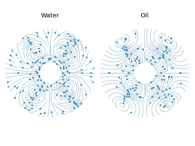
In this example we demonstrate how the microstreaming fields around the particle can be plotted from the model from Doinikov (2021).
 9 from matplotlib import pyplot as plt
10
11 import osaft
In this example we compare the streamlines around a polystyrene particle suspended in water and a polystyrene particle suspended in oil.
17 # -----------------
18 # Properties of Oil
19 # -----------------
20 # Speed of sound
21 c_oil = 1_400  # [m/s]
22 # Density
23 rho_oil = 900  # [kg/m^3]
24 # Shear viscosity
25 eta_oil = 0.04  # [Pa s]
26 # Bulk viscosity (neglected)
27 zeta_oil = 0  # [Pa s]
28
29 # -------------------
30 # Properties of Water
31 # -------------------
32 # Speed of sound
33 c_w = 1_498  # [m/s]
34 # Density
35 rho_w = 997  # [kg/m^3]
36 # Shear viscosity
37 eta_w = 0.0089  # [Pa s]
38 # Bulk viscosity (neglected)
39 zeta_w = 0  # [Pa s]
40
41 # --------------------------------------
42 # Properties of the polystyrene particle
43 # --------------------------------------
44 # Radius
45 R_0 = 5e-6  # [m]
46 # Density
47 rho_ps = 1_050  # [kg/m^3]
48 # Young's modulus
49 E_ps = 3.25e9  # [Pa]
50 # Poisson's ratio
51 nu_ps = 0.34  # [-]
52
53 # --------------------------------
54 # Properties of the acoustic field
55 # --------------------------------
56 # Frequency
57 f = 1e6  # [Hz]
58 # Wavetype
59 wt = osaft.WaveType.STANDING
60 # Position
61 h = 0  # [rad]
62 # Pressure amplitude
63 p_0 = 1e6  # [Pa]
For the plotting of streaming fields we use the StreamingField classes of the model doinikov2021viscous
69 doinikov_oil = osaft.doinikov2021viscous.StreamingField(
70     f=f, R_0=R_0,
71     rho_s=rho_ps, E_s=E_ps, nu_s=nu_ps,
72     rho_f=rho_oil, c_f=c_oil,
73     eta_f=eta_oil, zeta_f=zeta_oil,
74     p_0=p_0, wave_type=wt,
75     position=h,
76     N_max=3,
77 )
78
79 doinikov_water = osaft.doinikov2021viscous.ARF(
80     f=f, R_0=R_0,
81     rho_s=rho_ps, E_s=E_ps, nu_s=nu_ps,
82     rho_f=rho_w, c_f=c_w,
83     eta_f=eta_w, zeta_f=zeta_w,
84     p_0=p_0, wave_type=wt,
85     position=h,
86     N_max=3,
87 )
Analogous to the scattering field, the OSAFT library provides plotting method for the streamlines of the streamingfield.
 94 plot_water = osaft.FluidStreamingPlot(
 95     doinikov_water, r_max=4 * R_0,
 96 )
 97
 98 plot_oil = osaft.FluidStreamingPlot(
 99     doinikov_oil, r_max=4 * R_0,
100 )
101
102 if __name__ == '__main__':
103
104     fig, ax = plt.subplots(1, 2, subplot_kw={'projection': 'polar'})
105     plot_water.plot_streamlines(ax=ax[0])
106     plot_oil.plot_streamlines(ax=ax[1])
107
108     ax[0].set_title('Water')
109     ax[1].set_title('Oil')
110     fig.tight_layout()
111
112     plt.show()
Total running time of the script: ( 3 minutes 58.160 seconds)
Estimated memory usage: 10 MB