Note
Go to the end to download the full example code
Frontiers: HFE Droplet in Water
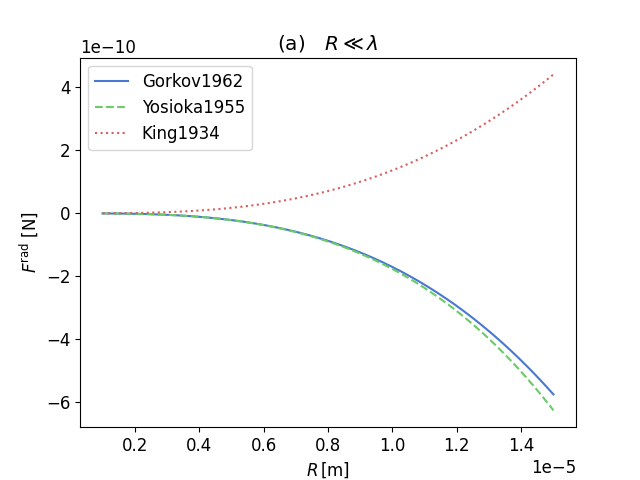
This example corresponds to section 3.2 in our publication. In this example we compute the acoustic radiation force (ARF) on a HFE droplet suspended in water subjected to a plane standing wave. We compare the theories from King (1934), Yosioka & Kawasima (1955), and Gor’kov (1962).
As always we start off by importing the nececassry Python modules. For this example we are going to need the osaft library, and the third party packages NumPy and Matplotlib.
18 import numpy as np
19 from matplotlib import pyplot as plt
20
21 import osaft
The next step is to define the properties for our example, these include the material properties, the properties of the acoustic field and the radius of the particle. In the osaft library we are always assuming SI-units..
The wave type is set using the osaft.WaveType enum. Currently, there are
two options:
osaft.WaveType.STANDING and osaft.WaveType.TRAVELLING for a plane
standing wave and a plane travelling wave, respectively.
35 # --------
36 # Geometry
37 # --------
38 # Radius
39 R_0 = 1e-6  # [m]
40
41 # -----------------
42 # Properties of HFE
43 # -----------------
44 # Speed of sound
45 c_hfe = 659  # [m/s]
46 # Density
47 rho_hfe = 1_621  # [kg/m^3]
48
49 # -------------------
50 # Properties of Water
51 # -------------------
52 # Speed of sound
53 c_w = 1_498  # [m/s]
54 # Density
55 rho_w = 997  # [kg/m^3]
56
57 # --------------------------------
58 # Properties of the Acoustic Field
59 # --------------------------------
60 # Frequency
61 f = 5e6  # [Hz]
62 # Pressure
63 p_0 = 1e5  # [Pa]
64 # Wave type
65 wave_type = osaft.WaveType.STANDING
66 # Position of the particle in the field
67 position = np.pi / 4  # [rad]
Once all properties are defined we can initialize the solution classes.
In this example, we use the classes osaft.king1934.ARF(),
osaft.yosioka1955.ARF(), and osaft.gorkov1962.ARF().
 75 # Theory of King
 76 king = osaft.king1934.ARF(
 77     f=f,
 78     R_0=R_0,
 79     rho_s=rho_hfe,
 80     rho_f=rho_w, c_f=c_w,
 81     p_0=p_0,
 82     wave_type=wave_type,
 83     position=position,
 84 )
 85
 86 # Theory of Yosioka
 87 yosioka = osaft.yosioka1955.ARF(
 88     f=f,
 89     R_0=R_0,
 90     rho_s=rho_hfe, c_s=c_hfe,
 91     rho_f=rho_w, c_f=c_w,
 92     p_0=p_0,
 93     wave_type=wave_type,
 94     position=position,
 95 )
 96
 97 # Theory of Gor'kov
 98 gorkov = osaft.gorkov1962.ARF(
 99     f=f,
100     R_0=R_0,
101     rho_s=rho_hfe, c_s=c_hfe,
102     rho_f=rho_w, c_f=c_w,
103     p_0=p_0,
104     wave_type=wave_type,
105     position=position,
106 )
First, want to evaluate the compressibility of the droplet and the fluid and the scattering coefficients \(f_1\) and \(f_2\). All these quantities are properties of the solution classes and can easily be evaluated.
116 # Compressibility
117 print(f'{yosioka.scatterer.kappa_f = :.2e}')
118 print(f'{yosioka.fluid.kappa_f = :.2e}')
119
120 # Gor'kov scattering coefficients
121 print(f'{gorkov.f_1 = :.2f}')
122 print(f'{gorkov.f_2 = :.2f}')
yosioka.scatterer.kappa_f = 1.42e-09
yosioka.fluid.kappa_f = 4.47e-10
gorkov.f_1 = -2.18
gorkov.f_2 = 0.29
Next, we want to compare the ARF from the different
theories in the small particle limit. To plot the ARF
we need to initialize an osaft.ARFPlot() instance.
With the method add_solutions() we can add our models to the instance.
With set_abscissa() we define the attribute that we want to
plot the ARF against. Here we select the radius R_0.
Finally, osaft.ARFPlot.plot_solutions() will generate the plot.
plot_solutions() returns two Matplotlib objects, a Figure and
an Axes object. These can be used to further manipulate the plot and to
save it.
To display the plot we need to call plt.show()
138 arf_plot = osaft.ARFPlot()
139
140 # Add solutions to be plotted
141 arf_plot.add_solutions(gorkov, yosioka, king)
142
143 # Define independent plotting variable (in this case the radius)
144 arf_plot.set_abscissa(np.linspace(1e-6, 15e-6, 300), 'R_0')
145 fig, ax = arf_plot.plot_solutions()
146
147 # Setting the axis labels and the title
148 ax.set_xlabel(r'$R \, \mathrm{[m]}$')
149 ax.set_title(r'$\mathrm{(a)} \quad R \ll  \lambda$')
150
151 plt.show()
/home/docs/checkouts/readthedocs.org/user_builds/osaft/checkouts/patch-doinikov2021_streaming/osaft/plotting/datacontainers/arf_datacontainer.py:52: AssumptionWarning: Theory might not be valid anymore!
  self._arf = self._compute_arf_single_process(attr_name, values)
Note
It is only possible to plot the ARF against
properties that wrap an underlying PassiveVariable, i.e. an input
parameter of the model.
You can get a list of all input variables using the method
input_variables().
161 print(f'{gorkov.input_variables() = }')
162 print(f'{yosioka.input_variables() = }')
163 print(f'{king.input_variables() = }')
gorkov.input_variables() = ['position', 'p_0', 'wave_type', 'rho_s', 'c_s', 'rho_f', 'c_f', 'R_0', 'f']
yosioka.input_variables() = ['small_particle', 'bubble_solution', 'position', 'p_0', 'wave_type', 'rho_s', 'c_s', 'rho_f', 'c_f', 'R_0', 'f', 'N_max']
king.input_variables() = ['small_particle_limit', 'position', 'p_0', 'wave_type', 'rho_s', 'rho_f', 'c_f', 'R_0', 'f', 'N_max']
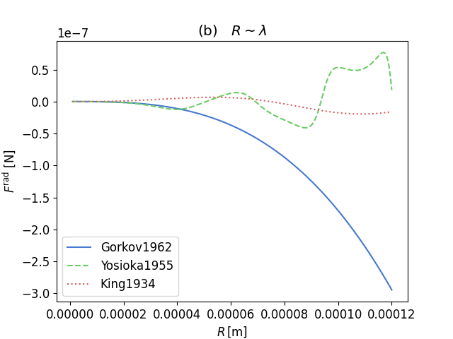
We redo our ARF plot, but this time the particle size is ranging from
1e-6 to 120e-6 meters.
169 # Plot
170 arf_plot.set_abscissa(np.linspace(1e-6, 120e-6, 300), 'R_0')
171 fig, ax = arf_plot.plot_solutions()
172
173 # Additional Matplotlib commands for the publication
174 ax.set_xlabel(r'$R \, \mathrm{[m]}$')
175 ax.set_title(r'$\mathrm{(b)} \quad R \sim  \lambda$')
176 plt.show()
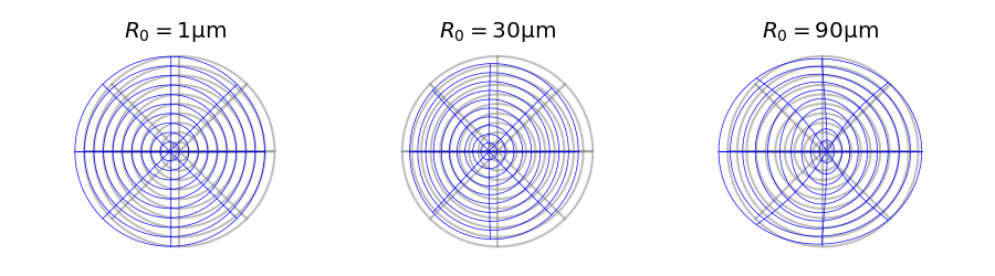
Lastly, we want to plot the mode shapes of the particle. We can do this
using the osaft.ParticleWireframePlot() class. To plot a specific model
we have to pass this model when initializing ParticleWireframePlot. We
can also pass a value for the scale_factor. The displacements in the
mode shape plot are exaggerated, the scale_factor is the ratio between
the maximal displacement and the particle radius in the exaggerated plot.
In our example we plot the mode shape for three different radii. Again,
we call plt.show() to display the plot.
191 # Creating a figure with subplots
192 fig, axes = plt.subplots(
193     1, 3, figsize=(9, 2.5), gridspec_kw={
194         'width_ratios':
195         [1, 1, 1],
196     },
197 )
198
199 # List of radii
200 radii = [1e-6, 30e-6, 90e-6]
201
202 # We loop through the three radii and the three subplots
203 for radius, ax in zip(radii, axes):
204
205     # During each loop we change the radius in the model
206     yosioka.R_0 = radius
207
208     # We plot the wireframe plot in the respect
209     wireframe_plot = osaft.ParticleWireframePlot(yosioka, scale_factor=0.1)
210     wireframe_plot.plot(ax=ax)
211
212     # Making the plot prettier
213     um_r = int(yosioka.R_0 * 1e6)
214     ax.axis(False)
215     ax.set_aspect(1)
216     ax.set_title(fr'$R_0 = {{{um_r}}}\mathrm{{\mu m}}$')
217
218 fig.tight_layout()
219 plt.show()
Total running time of the script: ( 0 minutes 5.000 seconds)
Estimated memory usage: 9 MB