Note
Go to the end to download the full example code
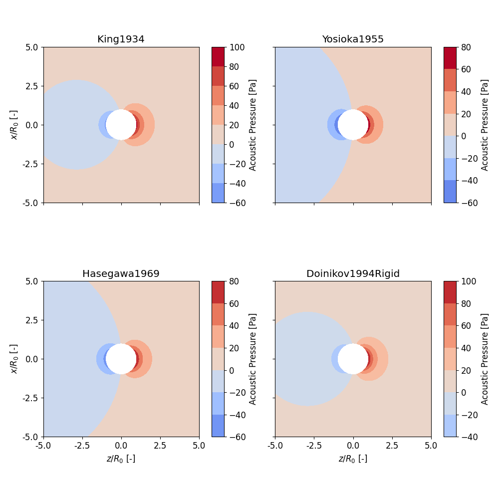
Pressure Plots for different theories
This example shows how to plot the pressure field for different theories in one single figure.
In this example we are investigating a polystyrene particle in a viscous oil in a standing wave.
13 from matplotlib import pyplot as plt
14
15 import osaft
16
17 # --------
18 # Geometry
19 # --------
20 # Radius
21 R_0 = 5e-6  # [m]
22
23 # -------------------------
24 # Properties of polystyrene
25 # -------------------------
26 # Density
27 rho_ps = 1_050  # [kg/m^3]
28 # Young's modulus
29 E_ps = 3.25e9  # [Pa]
30 # Poisson's ratio
31 nu_ps = 0.34  # [-]
32 # Speed of sound (matching compressibility)
33 c_ps = (E_ps / (rho_ps * 3 * (1 - 2 * nu_ps)))**0.5  # [m/s]
34
35 # -------------------
36 # Properties of Oil
37 # -------------------
38 # Density
39 rho_oil = 923  # [kg/m^3]
40 # Speed of sound
41 c_oil = 1_445  # [m/s]
42 # Viscosity
43 eta_oil = 0.03  # [Pa s]
44 zeta_oil = 0  # [Pa s]
45
46 # --------------------------------
47 # Properties of the Acoustic Field
48 # --------------------------------
49 # Frequency
50 f = 1e6  # [Hz]
51 # Pressure
52 p_0 = 1e5  # [Pa]
53 # Wave type
54 wave_type = osaft.WaveType.STANDING
55 # position
56 position = osaft.pi / 4
Once all properties are defined we can initialize the solution instances for the scattering field. We also save the solutions to a list which will make looping in the next steps straightforward.
 63 solutions = []
 64
 65 solutions.append(
 66     osaft.king1934.ScatteringField(
 67         f=f,
 68         R_0=R_0,
 69         rho_s=rho_ps,
 70         rho_f=rho_oil, c_f=c_oil,
 71         p_0=p_0,
 72         wave_type=wave_type,
 73         position=position,
 74     ),
 75 )
 76
 77
 78 solutions.append(
 79     osaft.yosioka1955.ScatteringField(
 80         f=f,
 81         R_0=R_0,
 82         rho_s=rho_ps, c_s=c_ps,
 83         rho_f=rho_oil, c_f=c_oil,
 84         p_0=p_0,
 85         wave_type=wave_type,
 86         position=position,
 87     ),
 88 )
 89
 90 solutions.append(
 91     osaft.hasegawa1969.ScatteringField(
 92         f=f,
 93         R_0=R_0,
 94         rho_s=rho_ps,
 95         E_s=E_ps, nu_s=nu_ps,
 96         rho_f=rho_oil, c_f=c_oil,
 97         p_0=p_0,
 98         wave_type=wave_type,
 99         position=position,
100     ),
101 )
102
103 solutions.append(
104     osaft.doinikov1994rigid.ScatteringField(
105         f=f,
106         R_0=R_0,
107         rho_s=rho_ps,
108         rho_f=rho_oil, c_f=c_oil,
109         eta_f=eta_oil, zeta_f=zeta_oil,
110         p_0=p_0,
111         wave_type=wave_type,
112         position=position,
113     ),
114 )
The next step is to initialise the plotter. We need a separate plotter for all solutions. We can now make use of the list of solutions. The respective plotters will be saved in a dictionary where the key is the name of the solution.
122 plotter = {}
123 for solution in solutions:
124     plotter[solution.name] = osaft.FluidScatteringPlot(
125         solution,
126         r_max=5 * solution.R_0,
127     )
Now we initialise an empty figure with four subplots and pass the
plt.Axes object to the plotting function. Additionally, we will also
change the title of the subplot.
136 fig, axes = plt.subplots(
137     nrows=2, ncols=2, figsize=(10, 10),
138     sharex=True, sharey=True,
139 )
140
141 count = 0
142 for name, plotter in plotter.items():
143     ax = axes.flat[count]
144     plotter.plot_pressure(
145         inst=True, incident=False, scattered=True, ax=ax,
146     )
147     ax.set_title(name)
148
149     # remove the y and x label for non-boundary subplots
150     if count == 0:  # top left
151         ax.set_xlabel('')
152     elif count == 1:  # top right
153         ax.set_xlabel('')
154         ax.set_ylabel('')
155     elif count == 3:  # bottom right
156         ax.set_ylabel('')
157
158     count += 1
159
160 fig.tight_layout()
161 plt.show()
Total running time of the script: ( 0 minutes 2.716 seconds)
Estimated memory usage: 9 MB