Frontiers: Copper Particle in Viscous Oil

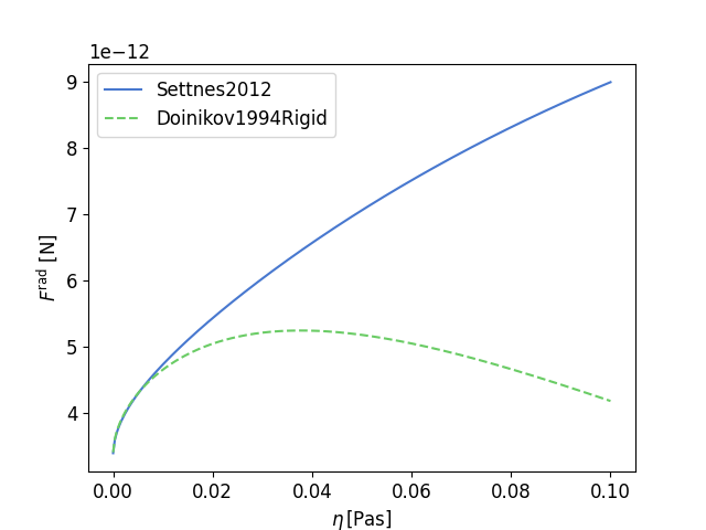
This example corresponds to section 3.3 in our publication. In this example we study the acoustic radiation force (ARF) on a copper particle suspended in a viscous oil. We compare the theory by Doinikov (rigid, 1994) and the theory by Settnes & Bruus (2012).

As always we start off by importing the necessary Python modules. For our example we are going to need the osaft library, and the packages NumPy and Matplotlib.

import numpy as np
from matplotlib import pyplot as plt
from matplotlib.patches import Circle

import osaft

The next step is to define the properties for our example, these include the material properties, the properties of the acoustic field and the radius. We always assume SI-units.

The wave type is set using the osaft.WaveType enum. Currently, there are two options: osaft.WaveType.STANDING and osaft.WaveType.TRAVELLING for a plane standing wave and a plane travelling wave, respectively.

# --------
# Geometry
# --------
# Radius
R_0 = 5e-6  # [m]

# --------------------
# Properties of Copper
# --------------------
# Speed of sound
rho_cu = 8_930  # [m/s]
# Density
c_cu = 5_100  # [kg/m^3]

# -------------------
# Properties of Oil
# -------------------
# Speed of sound
c_oil = 1_445  # [m/s]
# Density
rho_oil = 922.6  # [kg/m^3]
# Viscosity
eta_oil = 0.03  # [Pa s]
zeta_oil = 0  # [Pa s]

# --------------------------------
# Properties of the Acoustic Field
# --------------------------------
# Frequency
f = 5e5  # [Hz]
# Pressure
p_0 = 1e5  # [Pa]
# Wave type
wave_type = osaft.WaveType.STANDING
# Position of the particle in the field
position = np.pi / 4  # [rad]

# Once all properties are defined we can initialize the solution classes.
# In this example, we use the classes ``osaft.doinikov1994rigid.ARF()``, and
# ``osaft.settnes2012.ARF()``.

doinikov = osaft.doinikov1994rigid.ARF(
    f=f, R_0=R_0,
    rho_s=rho_cu,
    rho_f=rho_oil, c_f=c_oil,
    eta_f=eta_oil,
    zeta_f=zeta_oil, p_0=p_0, wave_type=wave_type,
    position=position, long_wavelength=True,
)

settnes = osaft.settnes2012.ARF(
    f=f, R_0=R_0,
    rho_s=rho_cu, c_s=c_cu,
    rho_f=rho_oil, c_f=c_oil,
    eta_f=eta_oil,
    p_0=p_0, wave_type=wave_type,
    position=position,
)

Next, we want to compare the boundary layer thickness and the particle radius for the given parameter. Both quantities are properties of our solution classes and can easily be evaluated, and we can compute the ratio.

print(f'{settnes.delta / settnes.R_0 = :.2f}')

settnes.delta / settnes.R_0 = 0.91

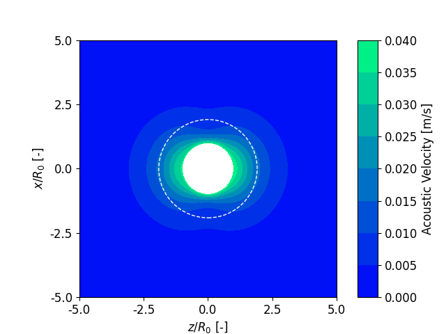
With the model from Doinikov it is also possible to compute the scattering field. To plot the scattering field we need to initialize a osaft.FluidScatteringPlot() instance. The class takes the model as an argument and the radius range r_max that is plotted. For more options see the documentation. The method plot() will then generate the plot. As always with Matplotlib, we need to call plt.show() to display the plot. plot() returns two Matplotlib objects, a Figure and an Axes object. These can be used to further manipulate the plot and to save it.

# Scattering plot small viscosity
scattering_plot = osaft.FluidScatteringPlot(doinikov, r_max=5 * doinikov.R_0)
fig, ax = scattering_plot.plot_velocity(inst=False, incident=False)

# Adding a circle to illustrate the boundary layer thickness
circle = Circle(
    (0, 0), doinikov.R_0 + doinikov.delta, fill=False,
    edgecolor='white', linestyle='--',
)
ax.add_artist(circle)
plt.show()

Finally, we want to compare the ARF in the different models. To plot the ARF we need to initialize an osaft.ARFPlot() instance. With the method add_solutions() we can add our models to the plotter. With set_abscissa() we define the variable that we want to plot the ARF against. Here we select the fluid viscosity eta_f. Finally, osaft.ARFPlot.plot_solutions() will generate the plot. Again, we call plt.show() to display the plot.

# sphinx_gallery_thumbnail_number = -1

# Initializing plotting class
arf_plot = osaft.ARFPlot()

# Add solutions to be plotted
arf_plot.add_solutions(settnes, doinikov)

# Define independent plotting variable (in this case the fluid viscosity)
arf_plot.set_abscissa(np.linspace(1e-5, 0.1, 300), 'eta_f')
fig, ax = arf_plot.plot_solutions()

# Setting the axis labels
ax.set_xlabel(r'$\eta \, \mathrm{[Pa s]}$')

plt.show()

/home/docs/checkouts/readthedocs.org/user_builds/osaft/checkouts/patch-doinikov2021_streaming/osaft/plotting/datacontainers/arf_datacontainer.py:52: AssumptionWarning: Theory might not be valid anymore!
  self._arf = self._compute_arf_single_process(attr_name, values)

Note

It is only possible to plot the ARF against properties that wrap an underlying PassiveVariable, i.e. an input parameter of the model. You can get a list of all input variables using the method input_variables().

print(f'{doinikov.input_variables() = }')
print(f'{settnes.input_variables() = }')

doinikov.input_variables() = ['long_wavelength', 'fastened_sphere', 'rho_s', 'position', 'p_0', 'wave_type', 'rho_f', 'c_f', 'eta_f', 'zeta_f', 'R_0', 'f', 'N_max', 'small_boundary_layer', 'large_boundary_layer', 'background_streaming']
settnes.input_variables() = ['position', 'p_0', 'wave_type', 'rho_s', 'c_s', 'rho_f', 'c_f', 'eta_f', 'R_0', 'f']

Estimated memory usage: 9 MB