Doinikov 1994 Models

In this example the use of the models doinikov1994rigid and doinikov1994compressible is explained. For this purpose, we are revisiting the example of a copper particle in oil using the doinikov1994rigid model. If you are not familiar with this example you might want to start here.

import numpy as np
from matplotlib import pyplot as plt

import osaft

# --------
# Geometry
# --------
# Radius
R_0 = 5e-6  # [m]

# --------------------
# Properties of Copper
# --------------------
# Speed of sound
c_cu = 8_930  # [m/s]
# Density
rho_cu = 5_100  # [kg/m^3]

# -------------------
# Properties of Water
# -------------------
# Speed of sound
c_oil = 1_445  # [m/s]
# Density
rho_oil = 922.6  # [kg/m^3]
# Viscosity
eta_oil = 0.03  # [Pa s]
zeta_oil = 0  # [Pa s]

# --------------------------------
# Properties of the Acoustic Field
# --------------------------------
# Frequency
f = 5e5  # [Hz]
# Pressure
p_0 = 1e5  # [Pa]
# Wave type
wave_type = osaft.WaveType.STANDING
# Position of the particle in the field
position = np.pi / 4  # [rad]

In this example we are going to explain the different option available to the user when computing the ARF using the models doinikov1994rigid and doinikov1994compressible. These versions make different assumptions on the relative size of the particle radius \(R_0\), the boundary layer thickness \(\delta\), and the wavelength \(\lambda\). Alternatively, the dimensionless wavenumber \(x = k_f R_0\) and the dimensionless viscous wavenumber \(x_v = k_v R_0\) can be used to represent the different cases.

The different options are listed in the table below for the model doinikov1994rigid. The different options are accessible through the keyword arguments long_wavelength, small_boundary_layer, and large_boundary_layer in the OSAFT classes for the ARF.

Assumption	\(x, x_v\)-representation	long_wavelength	small_boundary_layer	large_boundary_layer
no assumptions	–	False	False	False
\(\lambda \gg R_0, R_0 \gg \delta\)	\(|x| \ll 1, |x| \ll |x_v|\)	True	False	False
\(\lambda \gg R_0 \gg \delta\)	\(|x| \ll 1 \ll |x_v|\)	True	True	False
\(\lambda \gg \delta \gg R_0\)	\(|x| \ll |x_v| \ll 1\)	True	False	True

For the model doinikov1994compressible there is no long_wavelength option. If small_boundary_layer or large_boundary_layer is selected, long wavelength is automatically assumed.

Assumption	\(x\), \(x_v\)-representation	small_boundary_layer	large_boundary_layer
no assumptions	–	False	False
\(\lambda \gg R_0 \gg \delta\)	\(|x| \ll 1 \ll |x_v|\)	True	False
\(\lambda \gg \delta \gg R_0\)	\(|x| \ll |x_v| \ll 1\)	False	True

# General case
general_sol = osaft.doinikov1994rigid.ARF(
    f=f, R_0=R_0,
    rho_s=rho_cu,
    rho_f=rho_oil, c_f=c_oil,
    eta_f=eta_oil,
    zeta_f=zeta_oil, p_0=p_0, wave_type=wave_type,
    position=position, long_wavelength=False,
)
general_sol.name = 'General'


# Long wavelength
long_lambda_sol = general_sol.copy()
long_lambda_sol.long_wavelength = True
long_lambda_sol.name = 'Long wavelength'

# Long wavelength, small boundary layer
small_delta_sol = long_lambda_sol.copy()
small_delta_sol.small_boundary_layer = True
small_delta_sol.name = 'Small boundary layer'

# Long wavelength, large boundary layer
large_delta_sol = long_lambda_sol.copy()
large_delta_sol.large_boundary_layer = True
large_delta_sol.name = 'Large boundary layer'

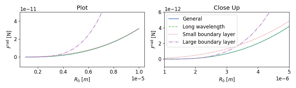
Note that the OSAFT library defaults to the general case, however the small particle solution might often be more sensible to use since it is computationally much more efficient and returns similar results over a wide range of values.

Next, we are going to plot the ARF over a range of values for the particle radius. Since computing the ARF in the general case requires solving integrals we are going to set the multicore option to True when adding solution. This way the ARF for different points are computed in parallel.

In order for multiprocessing to work you need to run your code inside the if __name__ == '__main__': clause as shown below. Check the multiprocessing example.

if __name__ == '__main__':

    arf_plot = osaft.ARFPlot('R_0', np.linspace(1e-6, 10e-6, 30))

    arf_plot.add_solutions(
        general_sol, long_lambda_sol,
        small_delta_sol, large_delta_sol,
        multicore=True,
    )

    fig, ax = plt.subplots(1, 2, figsize=(10, 3))

    arf_plot.plot_solutions(ax=ax[0])
    ax[0].set_xlabel('$R_0$ $[m]$')
    ax[0].set_ylim(top=0.5e-10)

    arf_plot.plot_solutions(ax=ax[1])
    ax[0].set_title('Plot')
    ax[1].set_title('Close Up')
    ax[1].set_xlabel('$R_0$ $[m]$')
    ax[1].set_xlim(left=1e-6, right=5e-6)
    ax[1].set_ylim(bottom=-1e-12, top=6e-12)
    ax[0].legend([], frameon=False)

    fig.tight_layout()
    plt.show()

Estimated memory usage: 9 MB